EDSAC, Dennis Wheeler and the Cambridge connection

Programmers everywhere, give thanks for EDSAC and David Wheeler, first implementer of the subroutine.

This month we return to the early days of modern computing. Specifically, to Cambridge (UK) in the late 1940s, and the first electronic digital stored-program computer to see regular service: the Electronic Delay Storage Automatic Calculator, or EDSAC (inspired by von Neumann’s First Draft of a Report on the EDVAC). The machine itself shared a lot of features with other computers of similar vintage, but it was while working on EDSAC that Dennis Wheeler developed the idea of subroutines and the first very basic assembler, making a contribution to computing that continues to this day.

EDSAC was constructed by Maurice Wilkes and his team at the University of Cambridge Mathematical Laboratory. It first ran in May 1949 and was immediately operational for research. Up in Manchester, the Mark I was first run in April 1949 but wasn’t running regularly or error-free until June 1949, so EDSAC beat it into regular service by a month.

EDSAC had mercury delay line memory, vacuum tubes for logic, punched-tape input and teleprinter output. Initially, there were 512 memory locations of 18 bits each available; later, in 1952, a further 512 locations came online. Timing issues meant that the first bit couldn’t be used, so an instruction consisted of a 5-bit instruction code, one unused bit, a 10-bit memory address, and a marker bit that identified whether the instruction was to operate on a number that was contained in one word or in two. This meant that EDSAC wasn’t restricted to 17-bit numbers but could also use 35-bit numbers contained in two words. Numbers were stored as binary two’s complement. The accumulator held 71 bits, so two 35-bit numbers could be multiplied without loss of precision. Initially it had only an accumulator and a multiplier registers — David Wheeler designed and added an index register in 1953.

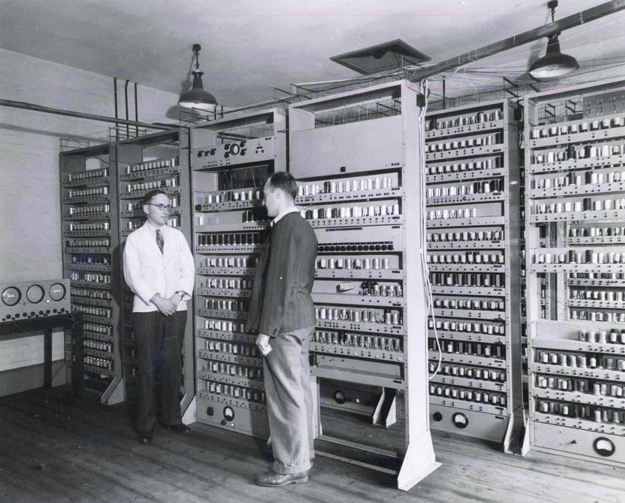
Bill Renwick (L) and Maurice Wilkes in front of the EDSAC I. Copyright Computer Laboratory, University of Cambridge. Reproduced by permission.

EDSAC and subroutines

David Wheeler (who earned the world’s first Computer Science PhD while working on EDSAC) was asked by Wilkes in 1949 to create a library of programs and subroutines for the machine. Grace Hopper was beginning to think about the same ideas at about this time, working on UNIVAC in the US. Wilkes and Hopper met when Wilkes visited the US in 1950, and Wilkes reported feeling that the two groups had much in common with how they thought about programming. In a 1958 paper by Hopper, she acknowledged that while subroutines had been a part of computing since the war years, the first real organisation and systematisation of them was done by the EDSAC group. The EDSAC library was certainly operational before Hopper’s UNIVAC libraries (and her A-0 ‘compiler’ which linked subroutines together) were. But clearly the notion of reusing code like this occurred to several people independently at about the same time – it’s a fairly obvious solution to a common problem, and early programmers were a resourceful bunch.

However, it was Wheeler who got there first; and a jump to subroutine is often still known as a Wheeler Jump. When the programmer called a Wheeler subroutine, the program would jump to the start of the subroutine with the address of the program counter plus one in the register. (So if it was at line 10, it would put line 11 into the register before jumping.) The subroutine would then write that address into its final line so it could jump back when it was finished. The user would have to copy the subroutine code into the right place on the tape. This demonstrates a technique used extensively by early programmers but which a modern coder would disapprove of: directly altering code to enable jumps and indexing.

By 1951, there were 87 subroutines available for EDSAC, covering a wide range of mostly mathematical operations, although print, layout, input, and loop simulation subroutines were also included.

Wheeler and the EDSAC team are also credited with the world’s first assembler, in the EDSAC’s Initial Orders 2. EDSAC’s instructions (see below) were designed to be represented by a mnemonic single letter (eg A for Add was coded using the bit pattern for A). The ‘initial orders’, setting up the basic operations for the machine, were hard-wired on switches and automatically loaded at startup into the first memory locations. EDSAC would then run from location 0. The first version of the initial orders was very basic, and in particular had the major limitation that all memory locations had to be absolute (ie referring to a numbered location).

The Initial Orders 2, written by Wheeler in May 1949, among other things enabled the programmer to refer to locations relative to a specified point, making it much easier to edit and debug programs. The Initial Orders 2 are fully described in the 1951 textbook The Preparation of Programs for an Electronic Digital Computer, by Wilkes, Wheeler, and Gill; this had a big impact on the programming culture of the 1950s, and its legacy lives on today. There’s also a listing of the Initial Orders in Martin Richard’s excellent poster at www.cl.cam.ac.uk/~mr10/Edsac/edsacposter.pdf.

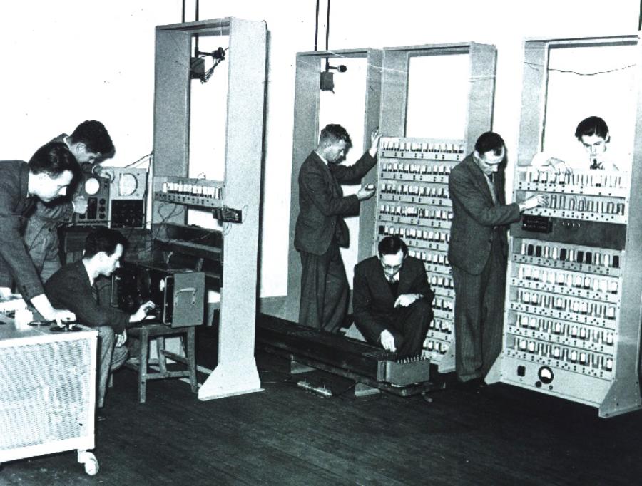
EDSAC may have been the site of the first video game – a version of noughts and crosses (tic-tac-toe) which output to the cathode ray tube. (The software is available for the simulator as oxo.txt.) Copyright Computer Laboratory, University of Cambridge. Reproduced by permission.

EDSAC emulator

Warwick University’s website (www.dcs.warwick.ac.uk/~edsac) has an EDSAC simulator for Linux. Unfortunately it’s very old (2002), so you may need to do a little fiddling to install it on a modern system. Using Debian (this should also work on Ubuntu; apologies to users of other distros), this is how I did it:

Click the Software menu item and download the Linux version of the software from that page.

Unzip and untar with tar zxf EdsacLX_v102.tar.gz.

Now cd into that directory. If you type ./runedsac you will most likely get a message telling you that the shared library libstdc++-libc6.1-1.so.2 cannot be found. This is a very old library which has been superseded.

The library can be found for Debian in the libstdc++2.9-glibc2.1_2.91.66-4_i386.deb package, available from http://archive.debian.net/woody/libstdc++2.9-glibc2.1. Download the Deb from that link (it advises you to use Aptitude but unless you wish to install lots of very old packages that seems like overkill to me).

Install the Deb with sudo dpkg -i libstdc+_-libc6.1-1.so.2.

Run the emulator with ./runedsac and this time all should be well.

NOTE: this is a very old, archived library package, which could have bugs or security risks. Install at your own risk. It might be sensible to uninstall it once you’re done playing with EDSAC, using dpkg -r. (With thanks to the debian-user list for the link.)

Let’s have a quick look at the emulator display panel Monitor display at left shows a single long tank (select which one with the Long Tank counter in the panel underneath). Bright dot for 1, small dot for 0. This represents a CRT display.

Output This represents the teleprinter output from a program.

Buttons These are mostly self-evident, but Single EP runs a program an instruction at a time. The Clear button was a slightly later addition. The original method of clearing the memory was, apparently, to earth the electrical terminals with a wet finger.

The clock represents ‘real time’ taken by the EDSAC. If you click the Real Time button in the top menu bar, the simulator will run in real time; otherwise it will run as fast as possible, but the clock will still show ‘EDSAC time’ to give you an idea of how fast (or not…) the original machine was.

Registers At bottom left are a representation of the registers (accumulator, multiplier, etc. In the real thing these were displayed on CRT tubes.

Dial This enables the operator to input a single decimal number.

The quickest way to see the emulator in operation is to run one of the included demo programs. For example, the Squares one, which is an exact copy of the Squares program run for the first time in 1949. To load it, click Clear, then choose Initial Orders 1 from the menu bar. Choose Open > Edsac Tapes > Demonstration Programs > Squares.txt, and the Squares file will pop up. Select Long Tank 0, then hit Start, and the initial orders, then the program, will load. You should soon see output on the teleprinter box. You can look at the various Long Tanks to see what is happening inside the machine.

The Tutorial Guide at the Warwick website
(www.dcs.warwick.ac.uk/~edsac/Software/EdsacTG.pdf) includes a full rundown of the Squares program, so we won’t reproduce that here (especially as it is very long). Instead, let’s try writing a much simpler program. To make life easier, we’re going to switch to using the Initial Orders 2 (change the drop-down box in the menu bar).

This program will output the numbers 1–5. Note that while I have added comments for ease of layout, these shouldn’t be typed into the program. However you can use new lines and spaces as you please. (Not historically accurate, but much simpler!) Save this as a .txt file.

T 64 K // Load the program in from instruction 64
G K // Set θ to current load point
Z F // Stop
O 9 @ //
O 10 @ //
O 11 @ //
O 12 @ // Print (output) location θ + 9 - 15
O 13 @ // (see below)
O 14 @ //
O 15 @ //
ZF // Stop
& F // Store linefeed
# F // Store figure shift
1 F // Store 1
2 F // Store 2
3 F // and so on
4 F
5 F
EZPF // Enter program at location θ

(With thanks to the Tutorial Guide.) F (which has the value 0) corresponds to S and D (value 1) to L in Initial Orders 2.

This loads the program from location 64 (which corresponds with the first line of long store 2, making it easy to find it and check that it has loaded correctly). It then sets the marker θ, and stops. The stop means that once we’ve loaded the program with the ‘Start’ button, we can check what it looks like before hitting ‘Reset’ to clear the Stop flag and continue with operations.

The next seven lines output locations θ + 9 to θ + 15. Instead of hard-coding a memory location, you set the θ marker, and then count lines from there. So θ + 9 is the line that contains & F; and so on. You store the data in one place and output it in another. The next ZF stops operation. After this we have the data storage. & is the line feed character, and # is the figure shift (* is the letter shift). You need to specify whether you’re outputting figures or letters in advance. We then store a bunch of numbers, and EZPF jumps back to θ and begins operation from there. (Which, in this instance, means an immediate Stop until the user hits Reset.)

Load and hit Start, and take a look at Long Tank 2. Then hit Reset to run the rest of the program and you should see the expected output. Try editing it by replacing #F with *F and output words instead.

If you try to edit this to output 1-6, you will notice that adding an extra line in the first part of the program means editing all the O lines. To avoid this, we can set another mark point. I’ve added line numbers for ease of reading but again, don’t include them in the file.

T 64 K // load at location 64
G K // Set θ mark
T 47 K // This loads label M
P 9 @ // and this places it at line θ + 9
T Z // Restore θ (ie set it here)
0 Z F // stop
1 O 0 M // output location M + 0
2 O 1 M // output location M + 1
.... O 2-6 M // and so on, as previous version
8 ZF // stop
M 0 & F // Store line feed
1 # F // Store figure shift
2 1 F // Store 1 ... and so on as before
EZPF // Start execution from θ

This has the same output as before, but instead of having to calculate “lines after θ” and alter them if you add more lines, you set the mark M (at a certain number of lines after θ) and then calculate data storage from there. If you add more lines before M, you only have to edit the P 9 @ line.

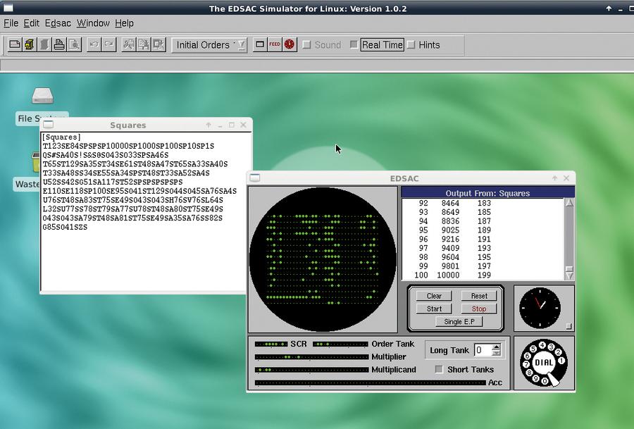
EDSAC simulator showing the final output of the Squares program. You can see from the dial that this took about six minutes to run.

Calculating Fibonacci numbers

Let’s try using a loop to calculate and output the Fibonacci sequence:

T 64 K // As above, this section reads in the program
G K // and sets θ
T 47 K // and these two lines
P 20 @ // set M
T Z // Reset θ
0 Z F // stop bell
1 O 0 M // output line feed
2 O 1 M // output figure shift
3 O 2 M // output 1st Fib number
4 O 0 M // lf
5 O 3 M // 2nd Fib number
6 O 0 M // lf
7 A 4 M // load number of rounds to run
8 T 4 M // transfer number of rounds out of accumulator and clear
9 A 2 M // load 1st Fib number into accumulator
10 A 3 M // add 2nd Fib number
11 U 3 M // transfer total into space for 2nd Fib number DO NOT clear
12 S 2 M // subtract original 1st from accumulator
13 T 2 M // transfer original 2nd into space for 1st
14 O 3 M // output new 2nd
15 O 0 M // lf
16 A 4 M // transfer number of rounds
17 S 5 M // subtract one round
18 E 8 @ // is number still positive? If so loop back to line 8
19 ZF // otherwise stop
M 0 & F // data! Line feed
1 # F // figure shift
2 1 F // 1st number
3 1 F // 2nd number
4 3 F // number of rounds
5 1 F // 1 -- for subtracting from rounds
EZPF // start from θ

The initial few lines are the program setup, as discussed above. Lines 1–7 output the initial ‘seed’ numbers of the sequence, and load the number of rounds to run. The main program loop is lines 8–18. We add the two seed numbers, store the result, and then move the 2nd of the seed numbers to the 1st storage position (line M2). As you’ll notice, this is done by subtracting #1 from the total (leaving #2) and storing the result in position #1. We now have the next two numbers ready for the next loop, and a cleared accumulator. We subtract one from the number of rounds, check whether it’s positive (note that 0 is positive, so you’ll get one more round than you might expect), and if it is, jump back to the start of the loop, where the number of rounds remaining is stored again. Once the number in M4 has reached -1, the program will stop (line 19).

Enter the program without line numbers and comments, then run it by hitting Clear, Start, and Reset to begin output, and you should get the first 6 Fibonacci numbers, as in the screenshot.

However, if you increase the value in line M4 and run it again, you’ll start getting weird output. This is because this output method only works for single digits. For larger numbers you’ll need to use the subroutine P6 to print them properly. Unfortunately there’s no space to look at that in this tutorial, but there’s plenty of information in the emulator’s Tutorial Guide if you want to extend this program, and it has a few suggested programming challenges. You can also examine the program listings included with the emulator software to learn more.

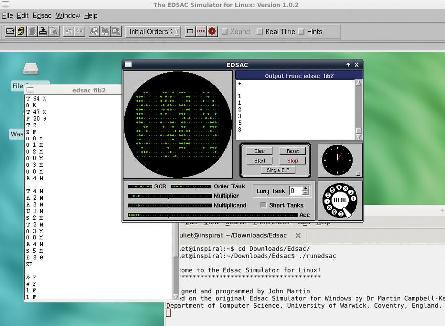
We’ve calculated the first six of the Fibonacci numbers, with the listing on left and the output showing in the teleprinter screen.

Other EDSAC tidbits

There is a collection of personal reminiscences from the program at the University of Cambridge Computer Laboratory webpage (www.cl.cam.ac.uk/events/EDSAC99/reminiscences). These include mention of the dissecting fluid smell of the EDSAC room (which was in what had been the anatomy school); memories of some of the technical experiments with magnetic tape; operational difficulties; and some recollections of the EDSAC summer schools (including one from Edsger Dijkstra).

Its successor, EDSAC 2, was commissioned in 1958; and in 1961 a version of Autocode (a high-level programming language a bit like ALGOL) was prodcued for EDSAC 2. Currently the Computer Conservation Society is building a working replica of EDSAC, to live at the National Museum of Computing at Bletchley Park, and hopes to have it operational by late 2015. See www.tnmoc.org/special-projects/edsac for more info.