Seymour Cray and the Development of Supercomputers
Join us in the Linux Voice time machine once more as we go back to the 1970s and the early Cray supercomputers.
Computers in the 1940s were vast, unreliable beasts built with vacuum tubes and mercury memory. Then came the 1950s, when transistors and magnetic memory allowed computers to become smaller, more reliable, and, importantly, faster. The quest for speed gave rise to the “supercomputer”, computers right at the edge of the possible in processing speed. Almost synonymous with supercomputing is Seymour Cray. For at least two decades, starting at Control Data Corporation in 1964, then at Cray Research and other companies, Cray computers were the fastest general-purpose computers in the world. And they’re still what many people think of when they imagine a supercomputer.
Seymour Cray was born in Wisconsin in 1925, and was interested in science and engineering from childhood. He was drafted as a radio operator towards the end of World War II, went back to college after the war, then joined Engineering Research Associates (ERA) in 1951. They were best known for their code-breaking work, with a little involvement with digital computing, and Cray moved into this area. He was involved in designing the ERA 1103, the first scientific computer to see commercial success. ERA was eventually bought out by Remington Rand and folded into the UNIVAC team.
In the late 1950s, Cray followed a number of other former ERA employees to the newly-formed Control Data Corporation (CDC) where he continued designing computers. However, he wasn’t interested in CDC’s main business of producing low-end commercial computers. What he wanted was to build the largest computer in the world. He started working on the CDC 6600, which was to become the first really commercially successful supercomputer. (The UK Atlas, operational at a similar time, only had three installations, although Ferranti was certainly interested in sales.)
Cray’s vital realisation was that supercomputing – computing power – wasn’t purely a factor of processor speed. What was needed was to design a whole system that worked as fast as possible, which meant (among other things) designing for faster IO bandwidth. Otherwise your lovely ultrafast processor would spend its time idly waiting for more data to come down the pipeline. Cray has been quoted as saying, “Anyone can build a fast CPU. The trick is to build a fast system.” He was also focussed on cooling systems (heat being one of the major problems when building any computer, even now), and on ensuring that signal arrivals were properly synchronised.
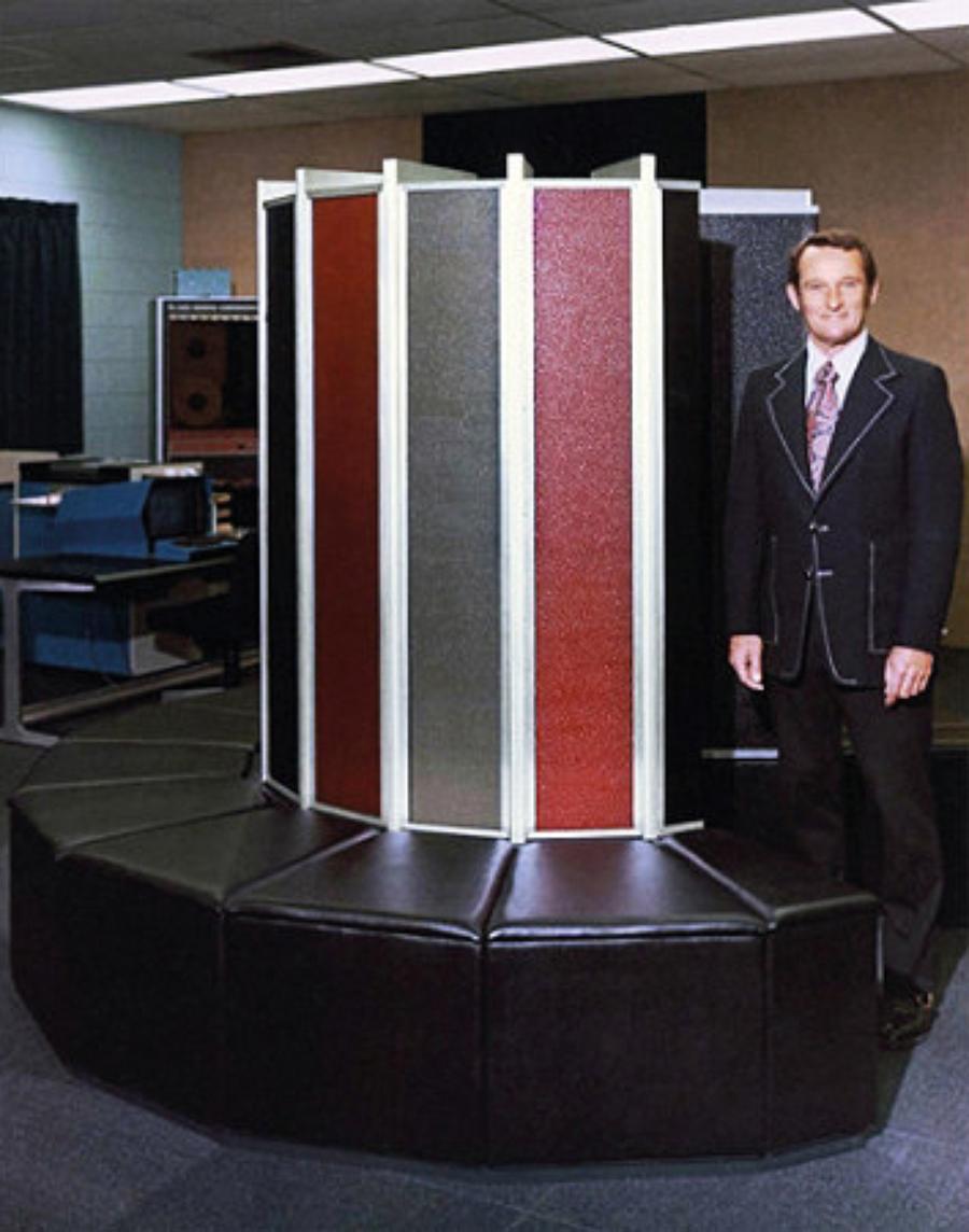
Seymour Cray with the Cray-1 (1976). Image courtesy of Cray Research, Inc.
CDC 6600: the first supercomputer
Cray made several big architectural improvements in the CDC 6600. The first was its significant instruction-level parallelism: it was built to operate in parallel in two different ways. Firstly, within the CPU, there were multiple functional units (execution units forming discrete parts of the CPU) which could operate in parallel; so it could begin the next instruction while still computing the current one, as long as the current one wasn’t required by the next. It also had an instruction cache of sorts to reduce the time the CPU spent waiting for the next instruction fetch result. Secondly, the CPU itself contained 10 parallel functional units (parallel processors, or PPs), so it could operate on ten different instructions simultaneously. This was unique for the time. The CPU read and decoded instructions from memory (via the PPs), and passed them onto the functional units to be processed. The CPU also contained an eight-word stack to hold previously executed instructions, making these instructions quicker to access as they required no memory fetch.
There were 10 PPs, but the CPU could only handle a single one at a time. They were housed in a ‘barrel’, and would be presented to the CPU one at a time. On each barrel ‘rotation’ the CPU would operate on the instruction in the next PP, and so on through each of the PPs and back to the start again. This meant that multiple instructions could be processing in parallel and the PPs could handle I/O while the CPU ran its arithmetic/logic independently. The CPU’s only connections to the PPs were memory, and a two-way connection such that either a PP could provide an interrupt, or it could monitor the central program address. To make best use of this, and of the functional units within the CPU, programmers had to write their code to take into account memory access and parallelisation of instructions, but the speed-up possibilities were significant.
A related improvement was in the size of the instruction set. At the time, it was usual to have large multi-task CPUs, with a large instruction set. This meant that they tended to run slowly. Cray, instead, used a small CPU with a small instruction set, handling only arithmetic and logic, which could therefore run much faster. For the other tasks usually dealt with by the CPU (memory access, I/O, and so on), Cray used secondary processors known as peripheral processors. Nearly all of the operating system, and all of the I/O (input/output) of the machine ran on these peripheral processors, to free up the CPU for user programs. This was the forerunner of the “reduced instruction set computing” (RISC) designs which gave rise to the ARM processor in the early 1980s.
The 6600 also had some instruction set idiosyncrasies. It had 8 general purpose X registers (60 bits wide), 8 A address registers (18 bits), and 8 B ‘increment’ registers (in which B0 was always zero, and B1 was often programmed as always 1) (18 bits). So far so normal; but instead of having an explicit memory access instruction, memory access was handled by the CPU as a side effect of assigning to particular registers (setting A1–A5 loaded the word at the given address into registers X1–X5, and setting A6 or A7 stored registers X6 or X7 into the given address). (This is quite elegant, really, but a little confusing at first glance.)
Physically, the machine was built in a + -shaped cabinet, with Freon circulating within the machine for cooling. The intersection of the + housed the interconnection cables, which were designed for minimum distance and thus maximum speed. The logic modules, each of two parallel circuit boards with components packed between them (cordwood construction) were very densely packed but had good heat removal. (Hard to repair though!) It had 400,000 transistors, over 100 miles of wiring, and a 100 nanosecond clock speed (the fastest in the world at the time). It also, of course, came with tape and disk units, high-speed card readers, a card punch, two circular ‘scopes’ (CRT screens) to watch data processing happening, and even a free operator’s chair.
Its performance was around 1 megaFLOPS, the fastest in the world by a factor of three. It remained the fastest between its introduction in 1964 (the first one went to CERN to analyse bubble-chamber tracks; the second one to Berkeley to analyse nuclear events, also inside a bubble chamber), and the introduction of the CDC 7600 in 1969. For more detail check out the book (written at the time) Design of a Computer: CDC6600 www.textfiles.com/bitsavers/pdf/cdc/6×00/books/DesignOfAComputer_CDC6600.pdf.
One important change in the Cray-1 was vector processing. This meant that if operating on a large dataset, instead of having an instruction for each member of the data set (ie looping round and swapping in a dataset member each time round the loop), the programmer could use a single instruction and apply it to the entire dataset. So instead of fetching a million instructions, the machine only fetches one. But more importantly, it also means that the CPU can use an ‘instruction pipeline’, queuing instructions up to be sent through the CPU while the previous one is still processing, rather than waiting for it to be fully completed.
Instruction pipelining wasn’t new — the 6600 did something rather like this, as did Atlas — but vector processors are able to fine-tune the pipelines because the data layout is known already to be a set of numbers arranged in order in a specific memory location. The Cray-1 took this a step further, using registers to load in a piece of data once and then apply, say, three operations to it, rather than processing the memory three times to operate on it three times. (Specifically, this was an improvement on the STAR.) This reduced flexibility, as registers were expensive to produce and therefore limited; the Cray-1 would have to read in a vector in portions of a particular size. However, the overhead was worth it in terms of the speed increase payoff. The Cray-1 hardware was optimised specifically to get these operations as fast as possible. Cray called this whole process “chaining”, as programmers could “chain” together instructions for performance improvements.
The Cray-1 was also the first Cray design to use integrated circuits (silicon chip style circuits) rather than wiring together a bunch of independent transistors. ICs were developed in the 1960s but initially were low-performance. By this time they had become fast enough to be worthwhile. However, they also ran very hot, especially in the huge stacks that were wired together for the Cray-1. (It had 1,662 modules each with one or two boards of up to 144 ICs per board.) The wiring was arranged so as to balance the load on the power supply very neatly. The circuit boards were paired with a copper sheet between them; the copper drew the heat to the outside where liquid Freon drew it away to the cooling unit. This system took some time to perfect as the lubricant and Freon mix kept leaking out of the seals.
The Cray-1 featured some other nifty tricks to get maximum speed – such as the shape of the chassis. The iconic C-shape was actually created to get shorter wires on the inside of the C, so that the most speed-dependent parts of the machine could be placed there, and signals between them speeded up slightly as they had less wire to get down. Overall throughput was around 4.5 times faster than the CDC 7600.
It was a 64 bit system (the 6600 and 7600 were 60-bit), with 24-bit addressing, and 1 megaword (ie 1M of 64-bit words) of main memory. It had eight 64-bit scalar registers and eight 24-bit address registers, each backed with 64 registers of temporary storage. In addition, the vector system had its own eight 64-element by 64-bit vector registers. There was also a clock register and 4 instruction buffers. Its fastest speed was around 250 MFLOPS, although in general it ran at around 160 MFLOPS.
Also it looked very cool, in a 1970s kind of way, with a central column, in orange and black, containing the processing unit, and a padded bench around it covering the power supplies. It weighed an impressive 5.5 tons (just shy of 5 metric tonnes), and used about 115kW of power (plus cooling and storage).
There’s a limit to what you can do on the simulator at the moment, but you could try running a test job, as described on Andras Tantos’ blog.
Cray-1
From 1968 to 1972, Cray was working on the CDC 8600, the next stage after the CDC 6600 and 7600. Effectively, this was four 7600s wired together; but by 1972 it was clear that it was simply too complex to work well. Cray wanted to start a redesign, but CDC was once again in financial trouble, and the money was not available. Cray, therefore, left CDC and started his own company, Cray Research very nearby. Their CTO found investment on Wall Street, and they were off again. Three years later, the Cray-1 was announced, and Los Alamos National Laboratory won the bidding war for the first machine.
They only expected to sell around a dozen, so priced them at around $8 million; but in the end they sold around 80, at prices of between $5 million and $8 million, making Cray Research a huge success. On top of that, users paid for the engineers to run it.
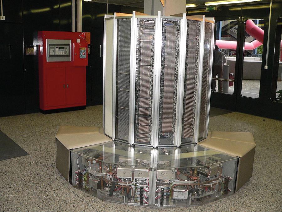
Cray-1 with its innards showing, in Lausanne. CREDIT/COPYRIGHT: CC-BY-SA 2.0 by Rama.
Emulators
Two awesome geeks, Chris Fenton and Andras Tantos, have been working on emulating the Cray-1. Chris’s project is to create a desktop size version, and the first part was (fairly) straightforward: build a model of the thing, and find a modern circuit board to hide inside it. Amazing though the Cray-1 was at the time, these days a tablet has more computing power.
But what Chris wanted was real Cray-1 software: specifically, COS. Turns out, no one has it. He managed to track down a couple of disk packs (vast 10lb ones), but then had to get something to read them… in the end he used an impressive home-brew robot solution to map the information, but that still left deciphering it. A Norwegian coder, Yngve Ådlandsvik, managed to play with the data set enough to figure out the data format and other bits and pieces, and wrote a data recovery script. Unfortunately that disk was just a maintenance image, but another disk was located which did indeed contain an OS image.
This is where Tantos came in; he found that the images were full of faults, so worked on a better recovery tool to reconstruct the boot disk. He’s been working on it since (his website has lots of detailed information and links to some of the disk images) and now has an emulator of sorts. In fact, it’s not strictly a Cray-1 but a Cray X-MP emulator. The Cray X-MP was an improvement on the Cray-1 design, released in 1982. Andras Tantos has lots of detailed information on it (http://modularcircuits.tantosonline.com/blog/articles/the-cray-files/the-return-of-the-cray). The other design path taken by Cray Research at the time led to the Cray-2, a full redesign which wasn’t particularly successful. As with all the Cray machines since, the instruction set of the Cray X-MP derives directly from the instruction set of the Cray-1. More pertinently, those were the disks that have been recovered, so that’s what we’ve got.
You can download the most recent zipfile from Tantos’ webpage (http://modularcircuits.tantosonline.com/blog/articles/the-cray-files/downloads). It has Windows binaries, but for Linux you’ll have to compile it yourself, as per these steps (on Debian stable up-to-date at time of writing):
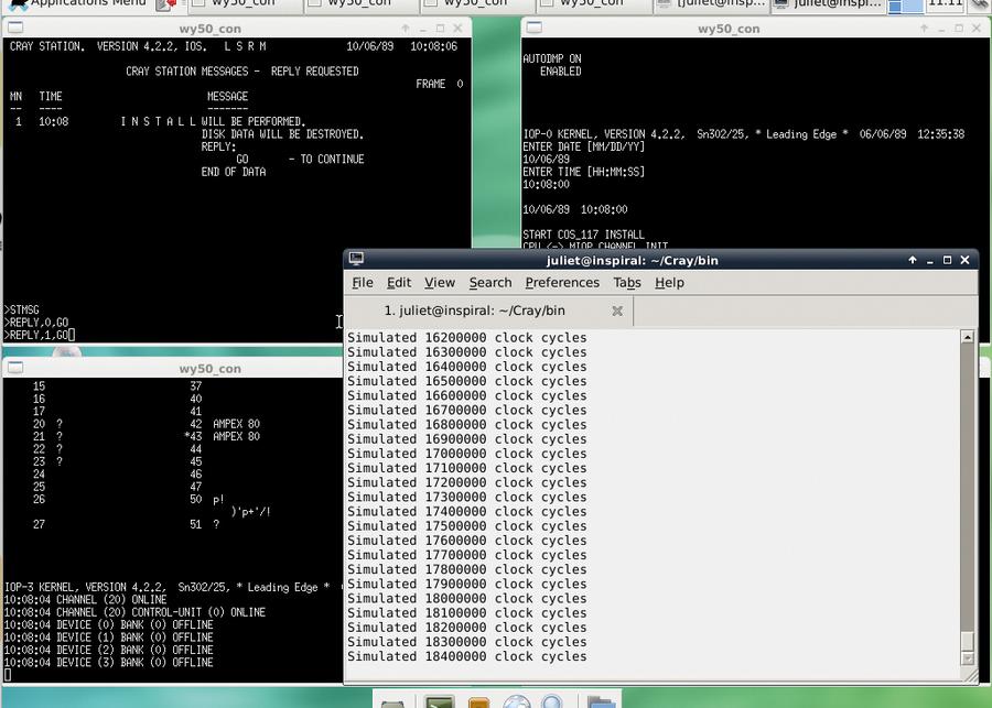
The emulator installing the system. The top-right window shows the ‘start’ commands, and the top-left is the station window.
Compile steps:
Install the Boost library (exists as Debian package libboost1.49-all-dev), GCC (gcc-4.7, g++-4.7, make, and libncurses5-dev).
Unzip the file into its own directory and cd into that directory, then add a line to sw/common.mak in the downloaded file, after the SYSTEM line (line 26):
SYSTEM=linux
SHELL=/bin/bash
Type make from the sw directory, and wait for a bit. (Tip: if you get an internal G++ compiler error, try increasing your swap.)
Copy the sw/_bin/linux_release files into bin/, then add ~/Cray/bin to your $PATH in .bashrc.
(With thanks to Jonathan Chin for assistance in fixing my compile problems. See also this page in French (http://framboisepi.fr/installation-dun-simulateur-cray) and Tantos’ instructions.)
You should now be ready to go. To start it up, cd bin and type cray_xmp_sim xmp_sim.cfg, and then follow the steps on Andras Tantos’ blog to get the system installed. Here’s a quick summary:
1 Enter a date and time (before 1999! Year-2000 error here…).
2 Type START COS_117 INSTALL.
3 Type STATION once you see the line
Concentrator ordinal 3 processed LOGON from ID FE
You’ll get a new window up: this is your main console (Cray Station) window. Type LOGON, then HELP to see the available commands.
4 To continue booting, type STMSG to see the system messages, then REPLY,0,GO to reply to message 0 and tell the system to GO.
5 When the next message pops up, warning that install is about to start, type REPLY,1, GO.
6 Installation takes 10–15 minutes on a fast machine. Go make a cup of tea. (Or try out some other commands, like STMSG,I to see the info messages.)
7 It’s done when FIXME gets this working!
When you’ve installed it once, you can use the deadstart process another time; please see Tantos’ blog for details.
Unfortunately, test jobs is all that you can do at the moment; there’s still no compiler, libraries, or any of the other parts of the system that would mean actually being able to write and run proper software. Tantos is still hopeful that something may show up, but sadly it is entirely possible that those disks are lost forever. Keep watching the project if you’re interested (and get in touch with him if anyone reading this happens to have a Cray disk in their loft!).
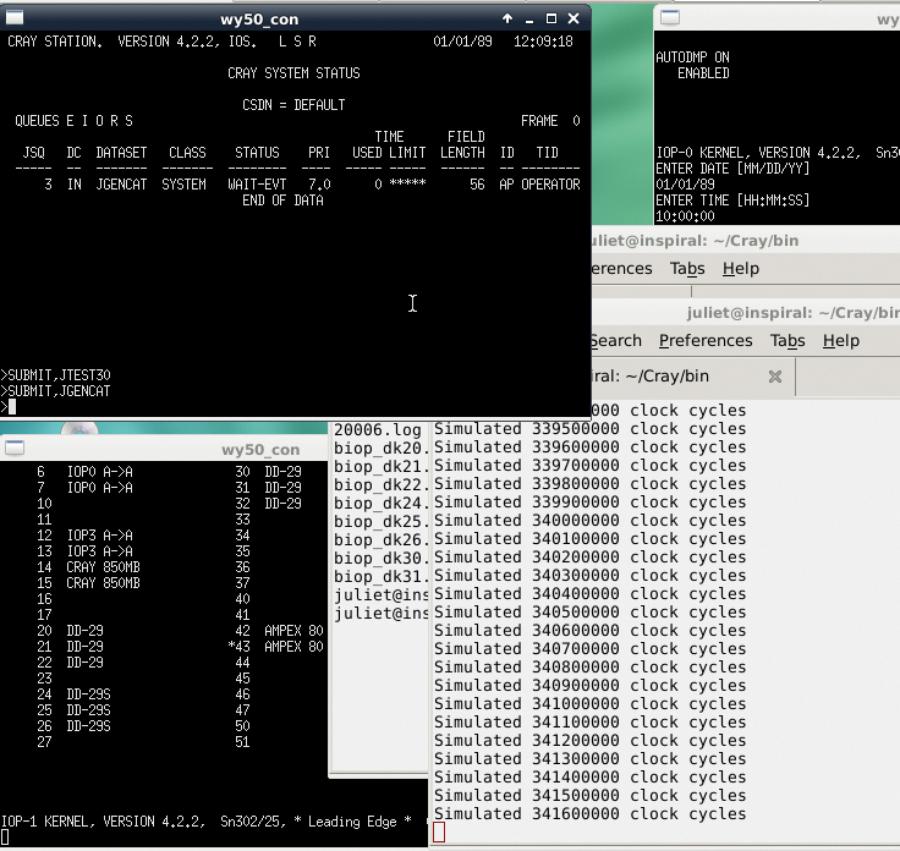
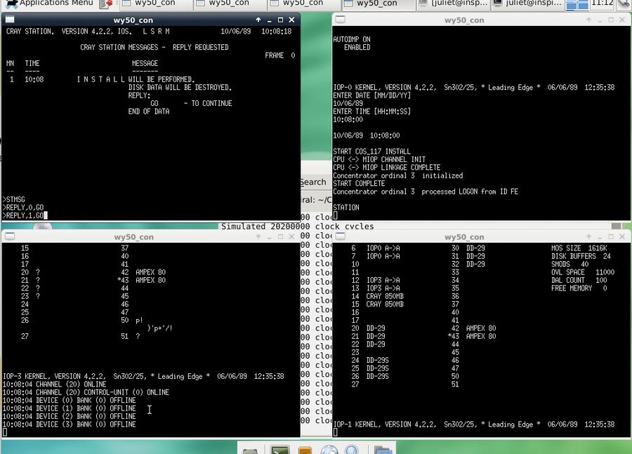
The Cray simulator running a job. The top-left window shows the status as the job is processed.
What happened next
Cray-related companies have gone through a multitude of mergers and separations over the years, and Seymour Cray died in a traffic accident in 1996. A company called Cray Inc does still exist, and as of Sept 2014 has just launched the XC40 and CS400 supercomputer and cluster supercomputer systems. These include SSD-based buffering with DataWarp, hoping to solve the current problem that compute power is increasing faster than regular disk-based IO can handle. It’s still very much in the game of designing whole system speed that Seymour Cray was so enthusiastic about.
Other emulators
There are a few other emulators online, though we haven’t tried them ourselves:
Verilog implementation of Cray-1 for FPGAs https://code.google.com/p/cray-1x/source/browse/#svn%2Ftrunk%2FSoftware.
Desktop CYBER emulator, which emulates various CDC machines but not the Cray-1 or others. It emulates the CDC 6400 but you need a disk image of your own to run an OS on it. http://members.iinet.net.au/~tom-hunter.
You can also log onto a real live Cray machine online, courtesy of the folks at www.cray-cyber.org. Unfortunately at time of writing this service was offline (while they’re moving their machines), but it is due back up soon. Many of the machines are only available on Saturdays as they cost so much to run (power bill donations are gratefully accepted). Sadly they don’t have a Cray-1 or Cray X-MP; all their Cray machines are later ones that run NOS.
Related Posts


About The Author
Juliet Kemp
Juliet is a scary polymath, and is the author of O’Reilly’s Linux System Administration Recipes. http://julietkemp.com